The Data Science of Predicting Disk Drive Failures

With the expanding volume of information in the digital universe and the increasing number of disk drives required to store that information, disk drive reliability prediction is imperative for EMC and EMC customers.

Figure 1- An illustration of the information expansion in the last years and expected growth

Disk drive reliability analysis, which is a general term for the monitoring and “learning” process of disk drive prior-to-failure patterns, is a highly explored domain both in academia and in the industry. The Holy Grail for any data storage company is to be able to accurately predict drive failures based on measurable performance metrics.

Naturally, improving the logistics of drive replacements is worth big money for the business. In addition, predicting that a drive will fail long enough in advance can facilitate product maintenance, operation and reliability, dramatically improving Total Customer Experience (TCE). In the last few months, EMC’s Data Science as a Service (DSaaS) team has been developing a solution capable of predicting the imminent failures of specific drives installed at customer sites.

Accuracy is key

Predicting drive failures is known to be a hard problem, requiring good data (exhaustive, clean and frequently sampled) to develop an accurate model. Well, how accurate should the developed model be? Very accurate! Since there are many more healthy drives than failed drives (a ratio of about 100:2 annually) the model has to be very precise when making a positive prediction in order to provide actual value.

EMC has been collecting telemetry on disk drives and other components for many years now, constantly improving the process efficacy. In a former project, we used drive error metrics collected from EMC VNX systems to develop a solution able to predict individual drive failures and thus avoid consecutive customer engineer visits to the same customer location (for more details contact the DSaaS team).  For the current proof of concept (POC) we used a dataset that BACKBLAZE, an online backup company, has released as open-source. This dataset includes S.M.A.R.T (Self-Monitoring, Analyses and Reporting Technology) measurements collected daily through 2015 from approximately 50,000 drives in their data center.  Developing the model on an open-source dataset makes it easier to validate the achieved performance and, equally important, allows for knowledge-sharing and for the “contribution” back to the community.

As of today, SMART attributes’ thresholds, which are the attributes values that should not be exceeded under normal operation, are set individually by manufacturers by means that are often considered a trade secret.  Since there are more than  100 SMART attributes (whose interpretation is not always consistent across vendors), rule-based learning of disk drive failure patterns is quite complicated and cumbersome, even without taking into account how different attributes affect each other (i.e. their correlations). Automated Machine Learning algorithms are very useful in dealing with these types of problems.

Implementation in mind

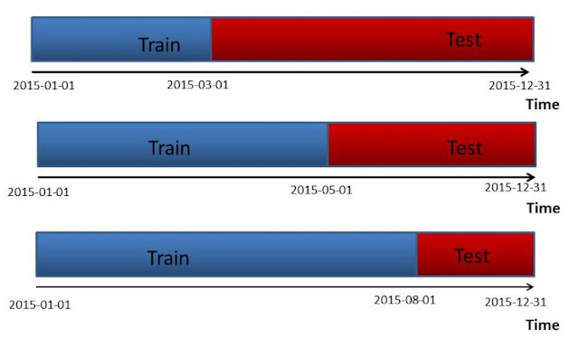
An important point to consider in this kind of analysis is that, unlike in a purely academic research, the solutions we are developing are meant to be either implemented in a product or as part of some business processes once their value is assessed in a POC. Thus, on each step of the modeling development process, we need to ask ourselves whether the tools and information we are using will be accessible when the solution is run in real time. To that end, we perform a temporal division of data into train and test sets. The division date can be set as a free parameter to the learning process, leaving room for different assignments and manipulations (several examples are illustrated in the plot below).  The critical point is that at the learning phase the model only has access to samples taken up to a certain date simulating the “current date” in a real-life scenario.

Figure 2- Examples of a temporal division of the data to train and test sets. The model can only learn from samples taken at the train period. The evaluation of the model is then performed on unseen samples taken in the test period.

In order to evaluate how well our solution can predict drive failures when applied on new data, we evaluate its performance solely on unseen samples taken at the test period. There are multiple performance metrics available such as model precision, recall and false positive rate. For this specific use case we are mainly looking to maximize the precision, which is the proportion of drives that will actually fail out of all the drives we predict as “going to fail.” Another measure of interest is how much time in advance we can predict a drive failure.  The accuracy of the provided solution and its extended scope into the future will have a direct effect on its eventual adoption by the business.

Engineering for informative features

At first, we only used the most recent sample from each drive for the model training. As we did not get accurate enough results (the initial precision was only 65 percent) we decided to add features describing longer time periods from the drive’s history. The more meaningful information we feed the model, the more accurate it will be. And since we have the daily samples taken over a year, why limit ourselves to the last sample only?

To picture the benefits of using a longer drive history, imagine yourself visiting the doctor and asking her for a full evaluation of your physical condition. She may run multiple tests and give you a diagnostic based solely on your physical measures on the current date, but these are subject to high variability- maybe today of all days is not a good representation of your overall condition. A more informative picture of your current state will be gained by running extensive, consecutive tests during continuous time-periods and look at all gathered data as a whole. In a sense, drives are like human beings- and we would like to capture and model their behavior over longer time periods.

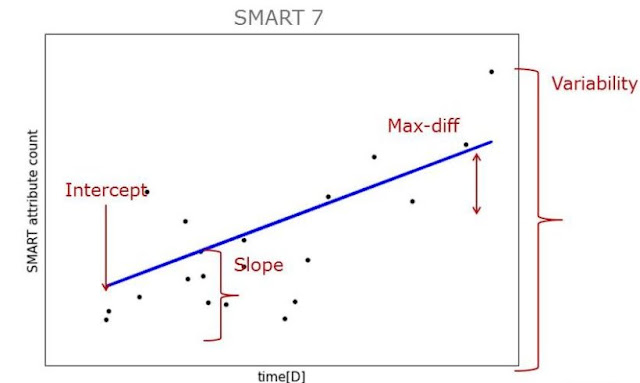
Most of the new calculated features capture different aspects concerned with the trend and rate of attribute change over time, as well as other statistical features of each attribute sample population. For example, we calculate the slope and intercept of the line that best describes the feature trend with time and the variance associated with each attribute at the specified time period.

Figure 3- Examples of features that can be extracted from the temporal ‘raw’ data, to capture the behavior of the drive in a continuous time window

We can choose the size of the measured time period according to our interest. For example, a reasonable choice would be to look at the drive’s behavior during two recent weeks or the last month. Once we have the new “historical” features, we can train a model whose predictions will be based on their values in addition to the original “raw” SMART attributes values.

Taking into account that the samples are collected daily, we use a “continuous” evaluation approach, such that we apply the model and acquire the predictions consecutively for each of the daily samples in the test period (see also figure 4 for an illustrative of the evaluation process). This allows us to update our knowledge regarding the state of the drive with the most recent data at our disposal.  Training and applying the model with the new “historical” features highly improve our results, increasing the precision to 83.3 percent, with a prediction mean time of 14 days prior to an actual failure.

Figure 4- A snapshot of the results for multiple runs of the trained model on samples taken in consecutive days of the evaluation period. These samples belong to a drive that failed during the test period and the figure depicts the evolution of model predictions as the drive approaches its failure date. The numbers and colors represent the assigned probability of the drive to fail with -1 in green representing already failed drives.